43 how to add percentage data labels in excel bar chart

How to show value and percentage in bar chart in excel The race bar chart is an animated bar chart , showing the development of an entity (usually top 10) over time The Progress Chart will look like this: Pre-requisites: To create this type of chart , we need to have data in the specific format Developed since 2006 Create Animated Charts When you to create a new project, to simplify the process of ... support.microsoft.com › en-us › officeAdd a pie chart - support.microsoft.com To switch to one of these pie charts, click the chart, and then on the Chart Tools Design tab, click Change Chart Type. When the Change Chart Type gallery opens, pick the one you want. See Also. Select data for a chart in Excel. Create a chart in Excel. Add a chart to your document in Word. Add a chart to your PowerPoint presentation

Progress Doughnut Chart with Conditional Formatting in Excel 24.03.2017 · The text boxes are linked to each cell in the data range for the chart. Free Chart Alignment Add-in. My FREE Chart Alignment Add-in allows you to move the chart elements (titles, labels, legend) with the arrow keys and alignment buttons. This can be very helpful and save time when building dashboards where we want the titles and labels to ...

How to add percentage data labels in excel bar chart

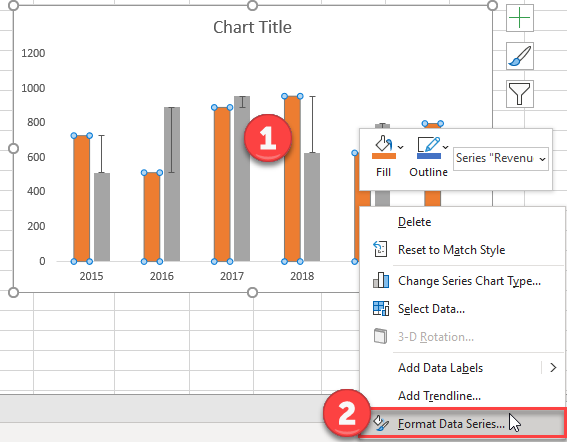
How to show data label in "percentage" instead of - Microsoft Community If so, right click one of the sections of the bars (should select that color across bar chart) Select Format Data Labels Select Number in the left column Select Percentage in the popup options In the Format code field set the number of decimal places required and click Add. HOW TO CREATE A BAR CHART WITH LABELS INSIDE BARS IN EXCEL - simplexCT 7. In the chart, right-click the Series "# Footballers" Data Labels and then, on the short-cut menu, click Format Data Labels. 8. In the Format Data Labels pane, under Label Options selected, set the Label Position to Inside End. 9. Next, in the chart, select the Series 2 Data Labels and then set the Label Position to Inside Base. Chart Axis - Use Text Instead of Numbers - Automate Excel Sales Funnel Chart: Floating Bar Chart: Forest Plot: Frequency Polygon: Arrow Chart: Percentage Graph: Time Series Graph: Percentage Change Chart: Show Percentage in Pie Chart: Dot Plot: Q-Q Plot: Log-Log Plot: Normal Probability Plot: Charts Tips & Tricks: yes: Add or Move Data Labels: Add Data Series: Add Average Line: Add Data Points: Add ...

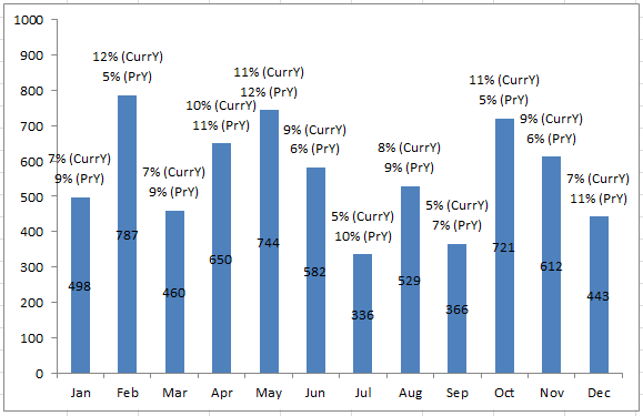
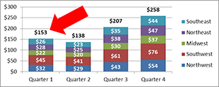
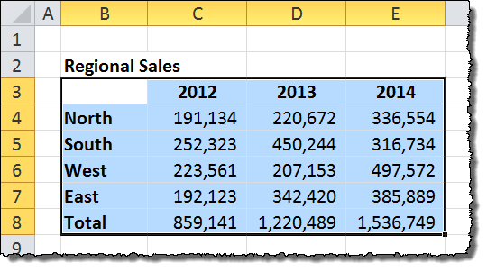
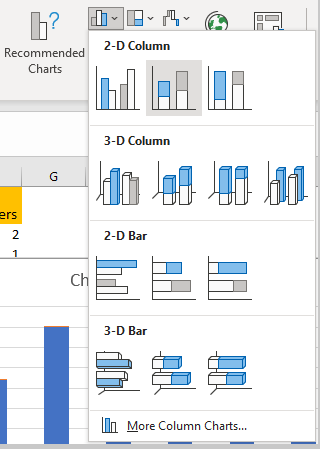
How to add percentage data labels in excel bar chart. How to create a chart with both percentage and value in Excel? Select the data range that you want to create a chart but exclude the percentage column, and then click Insert > Insert Column or Bar Chart > 2-D Clustered Column Chart, see screenshot: 2. Bar Chart - count & percentage - Microsoft Community To do this in Excel 2007: Click on a location within your chart so that the chart is activated and then from ribbon menu select the new contextual option Chart Tools. From here select the Layout tab and and then move over to the left side of the ribbon menu and you should see a drop down that says "Chart Area" or something else based on what ... How to show percentage in Bar chart in Powerpoint - Profit claims Steps to show Values and Percentage. 1. Select values placed in range B3:C6 and Insert a 2D Clustered Column Chart (Go to Insert Tab >> Column >> 2D Clustered Column Chart). See the image below. Insert 2D Clustered Column Chart2. In cell E3, type =C3*1.15 and paste the formula down till E6. Insert a formula3. support.microsoft.com › en-us › officeAdd or remove data labels in a chart - support.microsoft.com Click the data series or chart. To label one data point, after clicking the series, click that data point. In the upper right corner, next to the chart, click Add Chart Element > Data Labels. To change the location, click the arrow, and choose an option. If you want to show your data label inside a text bubble shape, click Data Callout.

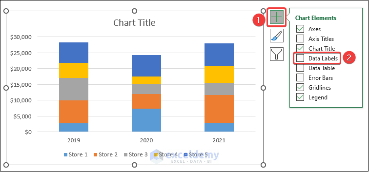
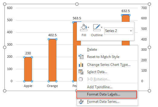
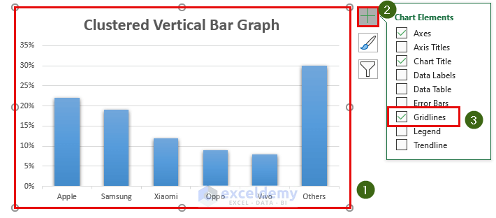
How to Show Percentage in Bar Chart in Excel (3 Handy Methods) - ExcelDemy 📌 Step 03: Add Percentage Labels Thirdly, go to Chart Element > Data Labels. Next, double-click on the label, following, type an Equal ( =) sign on the Formula Bar, and select the percentage value for that bar. In this case, we chose the C13 cell. Change the format of data labels in a chart To get there, after adding your data labels, select the data label to format, and then click Chart Elements > Data Labels > More Options. To go to the appropriate area, click one of the four icons ( Fill & Line, Effects, Size & Properties ( Layout & Properties in Outlook or Word), or Label Options) shown here. How to Make a Percentage Bar Graph in Excel (5 Methods) For the first method, we're going to use the Clustered Column to make a Percentage Bar Graph. Steps: Firstly, select the cell range C4:D10. Secondly, from the Insert tab >>> Insert Column or Bar Chart >>> select Clustered Column. This will bring Clustered vertical Bar Graph. How to Display Percentage in an Excel Graph (3 Methods) If you want to change the graph axis format from the numbers to percentages, then follow the steps below: First of all, select the cell ranges. Then go to the Insert tab from the main ribbon. From the Charts group, select any one of the graph samples. Now double click on the chart axis that you want to change to percentage.

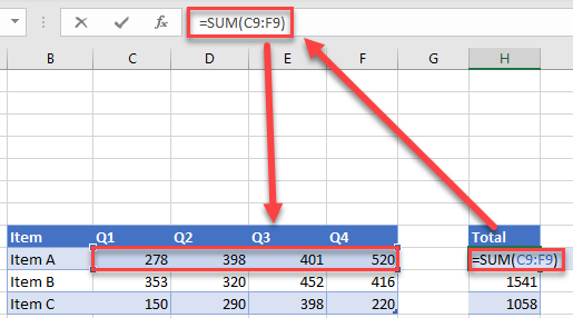
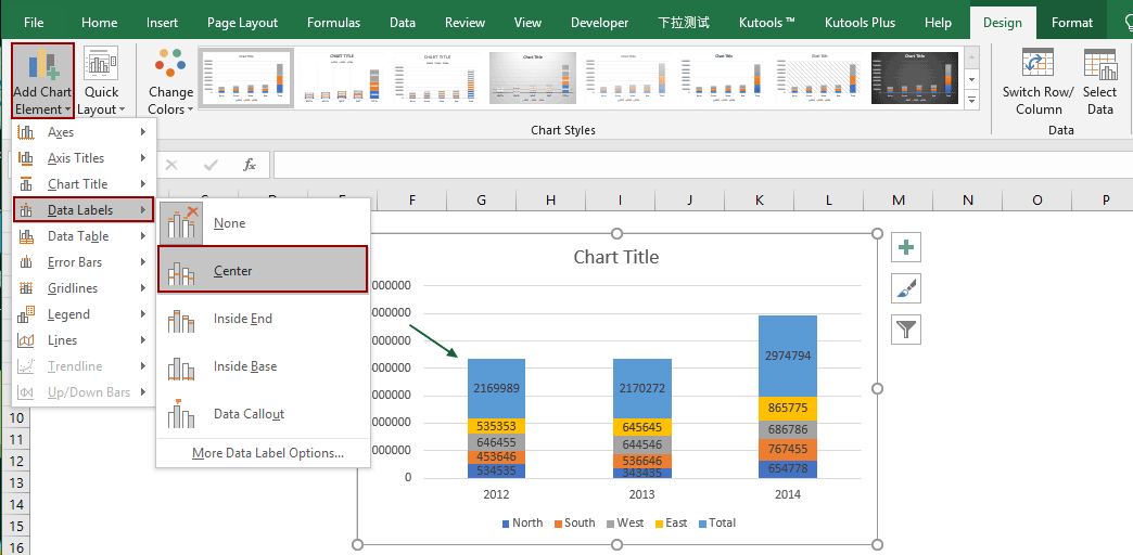
How to Add Percentage Axis to Chart in Excel We will click on the Numbers, then choose Percentage under Category: Our Chart now looks like this: Add Percentage Axis to Chart as Secondary. The above is a fairly easy example as we had only percentages to deal with. Now we want to present all of the data we have on one chart. Luckily, newer versions of Excel are pretty helpful in this regard. How to add total labels to stacked column chart in Excel? - ExtendOffice Select the source data, and click Insert > Insert Column or Bar Chart > Stacked Column. 2. Select the stacked column chart, and click Kutools > Charts > Chart Tools > Add Sum Labels to Chart. Then all total labels are added to every data point in the stacked column chart immediately. Create a stacked column chart with total labels in Excel How to Add Data Labels to an Excel 2010 Chart - dummies Use the following steps to add data labels to series in a chart: Click anywhere on the chart that you want to modify. On the Chart Tools Layout tab, click the Data Labels button in the Labels group. None: The default choice; it means you don't want to display data labels. Center to position the data labels in the middle of each data point. Legends in Chart | How To Add and Remove Legends In Excel Chart… A Legend is a representation of legend keys or entries on the plotted area of a chart or graph, which are linked to the data table of the chart or graph. By default, it may show on the bottom or right side of the chart. The data in a chart is organized with a combination of Series and Categories. Select the chart and choose filter then you will ...

Add Multiple Percentages Above Column Chart or Stacked Column ...

Count and Percentage in a Column Chart - ListenData Select Chart and click on "Select Data" button. Then click on Add button and Select E3: E6 in Series Values and Keep Series name blank. Select Data and Add Series: 5. In chart, select Second Bar (or Series 2 Bar) and right click on it and select Format Data Series and then check Secondary Axis under Plot Series On box in Series Options tab. Format Data Series: Change …

Change the format of data labels in a chart

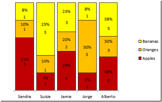
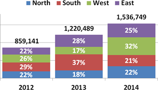
How to Show Percentages in Stacked Bar and Column Charts - Excel Tactics How to Show Percentages in Stacked Bar and Column Charts Quick Navigation 1 Building a Stacked Chart 2 Labeling the Stacked Column Chart 3 Fixing the Total Data Labels 4 Adding Percentages to the Stacked Column Chart 5 Adding Percentages Manually 6 Adding Percentages Automatically with an Add-In 7 Download the Stacked Chart Percentages Example File

How to show percentages in stacked column chart in Excel?

How to create progress bar chart in Excel? - ExtendOffice After installing Kutools for Excel, please do as this:. 1. Click Kutools > Charts > Progress > Progress Bar Chart, see screenshot:. 2.In the popped out Progress Bar Chart dialog box, please do the following operations:. Under the Axis label range, select the axis values from the original data;; Select Percentage of current completion option if you want to create the progress bar …

How to Add Totals to Stacked Charts for Readability - Excel ...

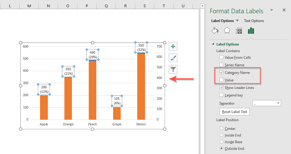
How to Add Two Data Labels in Excel Chart (with Easy Steps) For instance, you can show the number of units as well as categories in the data label. To do so, Select the data labels. Then right-click your mouse to bring the menu. Format Data Labels side-bar will appear. You will see many options available there. Check Category Name. Your chart will look like this.

Best Excel Tutorial - Chart with number and percentage

How to Add Percentages to Excel Bar Chart - Excel Tutorials Add Percentages to the Bar Chart If we would like to add percentages to our bar chart, we would need to have percentages in the table in the first place. We will create a column right to the column points in which we would divide the points of each player with the total points of all players. Our table will look like this:

How to Show Percentages in Stacked Bar and Column Charts in Excel

excel - How can I add chart data labels with percentage? - Stack Overflow I want to add chart data labels with percentage by default with Excel VBA. Here is my code for creating the chart: Private Sub CommandButton2_Click() ActiveSheet.Shapes.AddChart.Select ActiveChart. ... Programmatically adding excel data labels in a bar chart. 0. Painting a chart in Excel: conditional labels. 1. Add horizontal axis labels - VBA ...

Percentages as Labels for Stacked Bar Charts | SQL Server ...

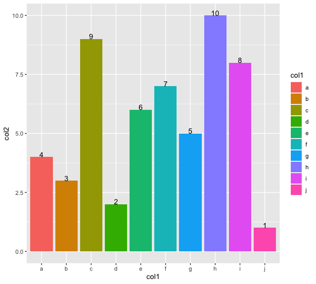
› 2016 › 06Count and Percentage in a Column Chart - ListenData Right Click on bar and click on Add Data Labels Button. 8. Right Click on bar and click on Format Data Labels Button and then uncheck Value and Check Category Name.

Friday Challenge Answer - Create a Percentage (%) and Value ...

Find, label and highlight a certain data point in Excel scatter graph 10.10.2018 · Add a new data series for the data point. With the source data ready, let's create a data point spotter. For this, we will have to add a new data series to our Excel scatter chart: Right-click any axis in your chart and click Select Data…. In the Select Data Source dialogue box, click the Add button. In the Edit Series window, do the following:

Make a Percentage Graph in Excel or Google Sheets – Automate ...

How to Create a Timeline Chart in Excel - Automate Excel In order to polish up the timeline chart, you can now add another set of data labels to track the progress made on each task at hand. Right-click on any of the columns representing Series “Hours Spent” and select “Add Data Labels.” Once there, right-click on any of the data labels and open the Format Data Labels task pane. Then, insert ...

How to Show Percentage in Bar Chart in Excel (3 Handy Methods)

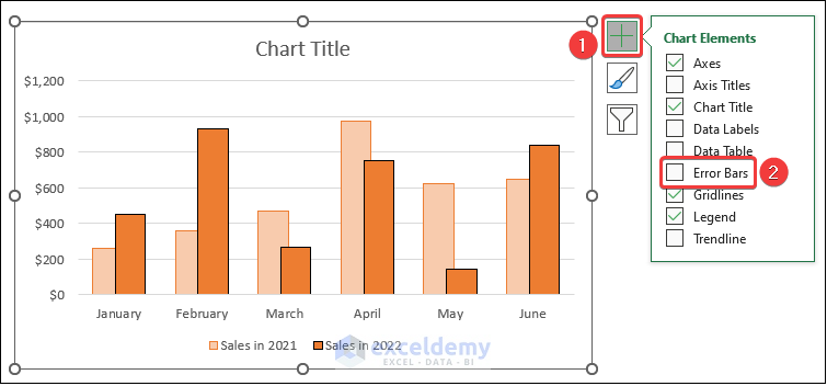
Create a column chart with percentage change in Excel - ExtendOffice Create a column chart with percentage change by using error bars Using the error bars to create a column chart with percentage change, you should insert some helper columns as below data shown, and then create the chart based on the helper data. Please do as follows: First, create the helper columns data 1.

Add Total Values for Stacked Column and Stacked Bar Charts in ...

› charts › axis-textChart Axis – Use Text Instead of Numbers - Automate Excel Select Change Chart Type . 3. Click on Combo. 4. Select Graph next to XY Chart. 5. Select Scatterplot . 6. Select Scatterplot Series. 7. Click Select Data . 8. Select XY Chart Series. 9. Click Edit . 10. Select X Value with the 0 Values and click OK. Change Labels. While clicking the new series, select the + Sign in the top right of the graph ...

Friday Challenge Answer - Create a Percentage (%) and Value ...

excel.officetuts.net › examples › add-percentageHow to Add Percentage Axis to Chart in Excel To do this, we will select the whole table again, and then go to Insert >> Charts >> 2-D Columns: To show percentages on a second axis, we first need to click anywhere on the orange bars that we have on our graph (this is not easy in this example as they are rather small). Once we do, we will right-click on it, and then select Format Data Series:

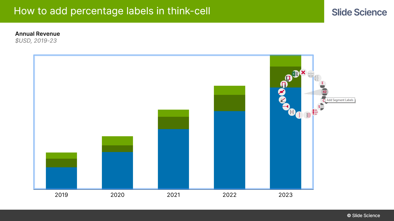
How to Add Percentage Labels in Think-Cell - Slide Science

› bar-chart-in-excelHow to Create Bar Chart in Excel? - EDUCBA Example #3. In this example, I am going to use a stacked bar chart. This chart tells the story of two series of data in a single bar. Step1: Set up the data first.I have the commission data for a sales team, which has been separated into two sections.

How to Show Percentage in Bar Chart in Excel (3 Handy Methods)

Data Bars in Excel (Examples) | How to Add Data Bars in Excel? - EDUCBA Data Bars in Excel is the combination of Data and Bar Chart inside the cell, which shows the percentage of selected data or where the selected value rests on the bars inside the cell. Data bar can be accessed from the Home menu ribbon's Conditional formatting option' drop-down list.

Excel: Clustered Column Chart with Percent of Month ...

Excel Charts: How To Show Percentages in Stacked Charts (in ... - YouTube Download the workbook here: the full Excel Dashboard course here: h...

How to Show Percentages in Stacked Bar and Column Charts in Excel

How to add percentage labels to top of bar charts? -Put a label "Year" in your source data -Select all your data -Create the chart bar/line chart -Then select the line part of the chart and right-click -Choose show data labels - then delete the line -finally place the % labels where you want them to be...

Format Number Options for Chart Data Labels in PowerPoint ...

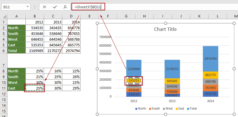
Showing percentages above bars on Excel column graph Use a line series to show the % Update the data labels above the bars to link back directly to other cells Method 2 by step add data-lables right-click the data lable goto the edit bar and type in a refence to a cell (C4 in this example) this changes the data lable from the defulat value (2000) to a linked cell with the 15% Share

How to Add Percentages to Excel Bar Chart – Excel Tutorials

HOW TO CREATE A BAR CHART WITH LABELS ABOVE BAR IN EXCEL - simplexCT In the Format Data Labels pane, under Label Options selected, set the Label Position to Inside End. 16. Next, while the labels are still selected, click on Text Options, and then click on the Textbox icon. 17. Uncheck the Wrap text in shape option and set all the Margins to zero. The chart should look like this: 18.

How to Make Pie Chart with Labels both Inside and Outside ...

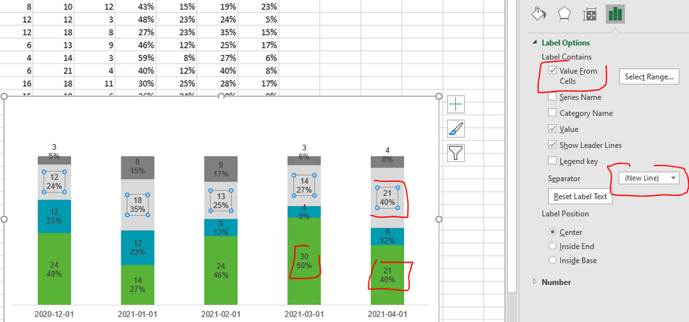
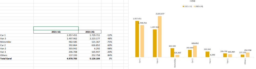
How can I show percentage change in a clustered bar chart? Double-click it to open the "Format Data Labels" window. Now select "Value From Cells" (see picture below; made on a Mac, but similar on PC). Then point the range to the list of percentages. If you want to have both the value and the percent change in the label, select both Value From Cells and Values. This will create a label like: -12% 1.729.711

How to create a chart with both percentage and value in Excel?

Quickly create a positive negative bar chart in Excel - ExtendOffice Now create the positive negative bar chart based on the data. 1. Select a blank cell, and click Insert > Insert Column or Bar Chart > Clustered Bar. 2. Right click at the blank chart, in the context menu, choose Select Data. 3. In the Select Data Source dialog, click Add button to open the Edit Series dialog.

How to Show Percentage in Pie Chart in Excel? - GeeksforGeeks

How to build a 100% stacked chart with percentages - Exceljet F4 three times will do the job. Now when I copy the formula throughout the table, we get the percentages we need. To add these to the chart, I need select the data labels for each series one at a time, then switch to "value from cells" under label options. Now we have a 100% stacked chart that shows the percentage breakdown in each column.

How to show percentages in stacked column chart in Excel?

Bar Chart in Excel (Examples) | How to Create Bar Chart in Excel? Bar Chart in Excel is one of the easiest types of the chart to prepare by just selecting the parameters and values available against them. We must have at least one value for each parameter. Bar Chart is shown horizontally, keeping their base of the bars at Y-Axis. Bar Chart can be accessed from the insert menu tab from the Charts section, which has different types of …

How to add percentage or count labels above percentage bar ...

› documents › excelQuickly create a positive negative bar chart in Excel Now create the positive negative bar chart based on the data. 1. Select a blank cell, and click Insert > Insert Column or Bar Chart > Clustered Bar. 2. Right click at the blank chart, in the context menu, choose Select Data. 3. In the Select Data Source dialog, click Add button to open the Edit Series dialog.

Percentage Change Chart – Excel – Automate Excel

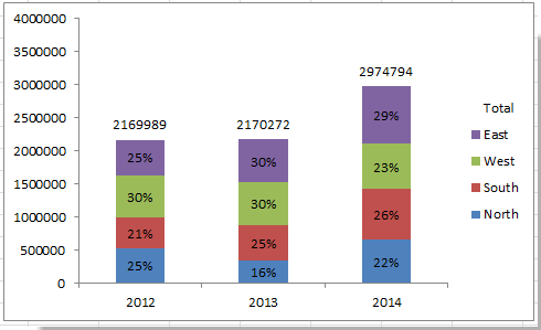
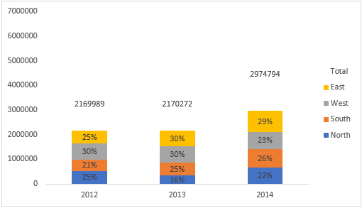
How to show percentages in stacked column ... - ExtendOffice Add percentages in stacked column chart 1. Select data range you need and click Insert > Column > Stacked Column. See screenshot: 2. Click at the column and then click Design > Switch Row/Column. 3. In Excel 2007, click Layout > Data Labels > Center . In Excel 2013 or the new version, click Design > Add Chart Element > Data Labels > Center. 4.

Solved: Clustered column chart - show percentage and value ...

How to Show Percentages in Stacked Column Chart in Excel? Follow the below steps to show percentages in stacked column chart In Excel: Step 1: Open excel and create a data table as below. Step 2: Select the entire data table. Step 3: To create a column chart in excel for your data table. Go to "Insert" >> "Column or Bar Chart" >> Select Stacked Column Chart. Step 4: Add Data labels to the chart.

How to show percentages in stacked column chart in Excel?

Chart Axis - Use Text Instead of Numbers - Automate Excel Sales Funnel Chart: Floating Bar Chart: Forest Plot: Frequency Polygon: Arrow Chart: Percentage Graph: Time Series Graph: Percentage Change Chart: Show Percentage in Pie Chart: Dot Plot: Q-Q Plot: Log-Log Plot: Normal Probability Plot: Charts Tips & Tricks: yes: Add or Move Data Labels: Add Data Series: Add Average Line: Add Data Points: Add ...

Solved: Display percentage in stacked column chart ...

HOW TO CREATE A BAR CHART WITH LABELS INSIDE BARS IN EXCEL - simplexCT 7. In the chart, right-click the Series "# Footballers" Data Labels and then, on the short-cut menu, click Format Data Labels. 8. In the Format Data Labels pane, under Label Options selected, set the Label Position to Inside End. 9. Next, in the chart, select the Series 2 Data Labels and then set the Label Position to Inside Base.